
T1
Technical Report · Systems

T1:面向长程任务的
终端 Agent 强化学习
T1: Terminal Agent Reinforcement
Learning for Long-horizon Tasks

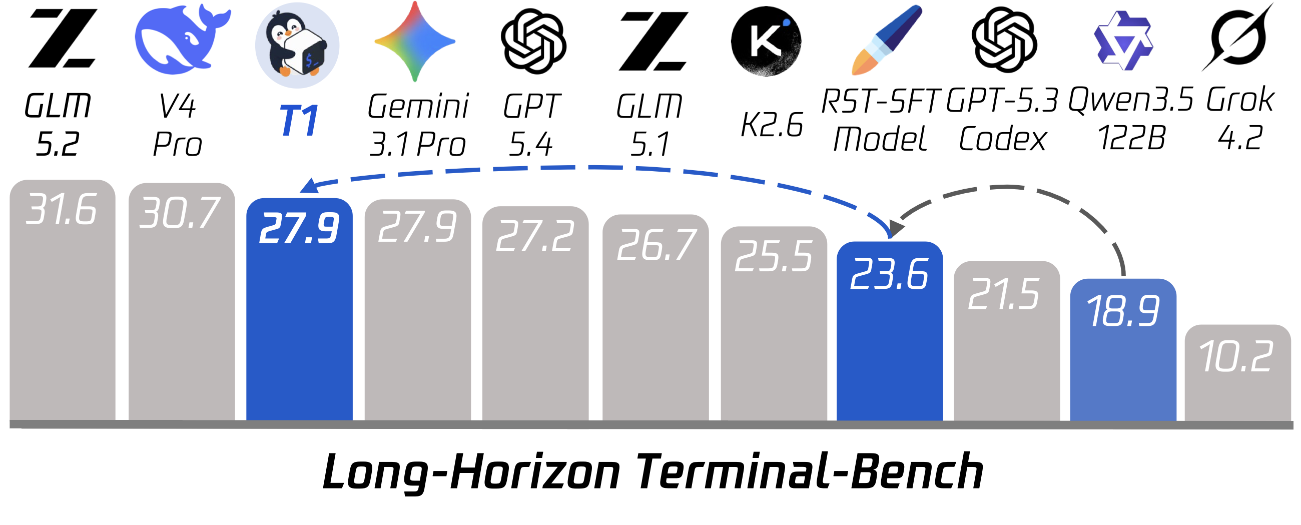
我们用强化学习把一个 122B-A10B 的 MoE 模型训练成能在云端沙箱里真正操作 Linux 终端的 Agent:单个任务最多 300+ 次工具调用,奖励直接来自任务自带测试套件的执行结果。 在 89 个留出任务的 Terminal-Bench 2.1 上,模型从 SFT 的 49.4% 提升到 64.0%, 在同一 harness 下超过 GPT-5.4 与 DeepSeek-V4-Flash,逼近 Claude Opus 4.7。

We post-train a 122B-A10B Mixture-of-Experts model with reinforcement learning to operate a real Linux shell inside a cloud sandbox — up to 300+ tool-call turns per task, rewarded by executing each task's own test suite. On Terminal-Bench 2.1 with 89 held-out tasks, RL raises our SFT model from 49.4% to 64.0% resolved, above GPT-5.4 and DeepSeek-V4-Flash and approaching Claude Opus 4.7 under the same harness.

64.0%
Terminal-Bench 2.1
(SFT 为 49.4%)
Terminal-Bench 2.1
(SFT: 49.4%)
122B-A10B
MoE 总参 / 激活参数MoE total / active params
+14.6pp
RL 相对 SFT 的净增益net gain of RL over SFT
97.4%
token 逐位对齐
损失区零漂移
tokens exactly aligned
zero drift in loss region

01为什么终端任务这么难Why terminal tasks are hard

Agent 的使用场景正在从简单的文件操作和对话问答,转向编程、科学发现这类长程任务,而 长程终端任务是其中格外重要的一类。我们的做法很直接:Agent 收到一段自然语言任务描述, 然后在一个隔离的云沙箱里反复"发命令 → 读输出",最多 60 个 assistant 轮次、单条轨迹数万 token; 最后由任务自带的 pytest 验证器在同一个沙箱里执行,给出奖励。

训练系统把 Megatron(训练)和 SGLang(推理)通过 slime v0.3 的 RL 框架连起来, Agent harness 用的是 Harbor / Terminus-2。所有 Agent 相关逻辑都放在插件层,而不是 fork 框架。 相比 RLHF 式或短答案式 RL,这个设定有三个本质困难:

Agent usage has shifted from simple file manipulation and conversational QA toward long-horizon tasks such as coding and scientific discovery, among which long-horizon terminal tasks stand out as a particularly important focus. Our setup is direct: the agent receives a natural-language task, then alternates between emitting shell commands and reading their output inside an isolated cloud sandbox, for up to 60 assistant turns and tens of thousands of tokens per trajectory. A trajectory is scored by executing the task's own pytest verifier inside the same sandbox.

The training system connects Megatron (training) and SGLang (inference) through the slime v0.3 RL framework, with the agent harness provided by Harbor / Terminus-2. All agent-specific logic lives in a plugin layer rather than a framework fork. Three properties make this setting substantially harder than RLHF-style or short-answer RL:

长程、工具交错的轨迹Long-horizon, tool-interleaved trajectories

训练序列会打到 64k–84k token 的墙,由多达 60 段模型/工具片段拼成,而只有模型生成的 token 才允许携带损失。每个轮次边界都是 harness 做「解码 → 解析 → 重新套模板 → 重新编码」往返的机会,一不小心训练器条件化的 token 序列就变了。

Training sequences reach the 64k–84k-token wall, are assembled from up to 60 alternating model/tool segments, and only model-generated tokens may carry loss. Every turn boundary is an opportunity for the harness's decode → parse → re-template → re-encode round trip to change the token sequence the trainer conditions on.

MoE 特有的训推不一致MoE-specific train–inference mismatch

专家权重占了总参数的 95.5%(116.0B / 121.4B),每个 token 在每层从 256 个专家里离散地选 8 个。推理栈和训练栈之间极小的数值差异就足以翻转这个离散选择——于是训练侧的前向可能把梯度送进了另一批参数

Expert weights are 116.0B of the 121.4B total parameters (95.5%), and each token engages 8 of 256 experts per layer via a discrete top-k router. Small numeric differences between the inference and training stacks can flip these discrete choices, so the training-side forward may route gradient through different parameters.

稀疏且昂贵的奖励Sparse, expensive reward

一个 rollout batch 要烧掉数百沙箱小时,而二值的「任务是否解决」只提供 1 bit 信息。我们第一次 122B RL(TMax 池 + 二值奖励)始终没能超过 SFT 基线。

A full rollout batch costs hundreds of sandbox-hours, while a binary task-solved reward provides one bit per trajectory. Our first 122B RL campaign (TMax pool, binary rewards) never exceeded the SFT baseline.

两条正交的修复轴Two orthogonal axes

token 漂移在序列层面破坏 PPO 的重要性比率,路由漂移在参数层面破坏它。我们把二者当成正交问题分别解决:TITO 管 token,R³ 路由回放管专家。

Token drift breaks PPO's importance ratio at the sequence level; routing divergence breaks it at the parameter level. We treat these as orthogonal and fix them separately: TITO for tokens, R³ routing replay for experts.

Model size versus Terminal-Bench 2.1 resolved rate
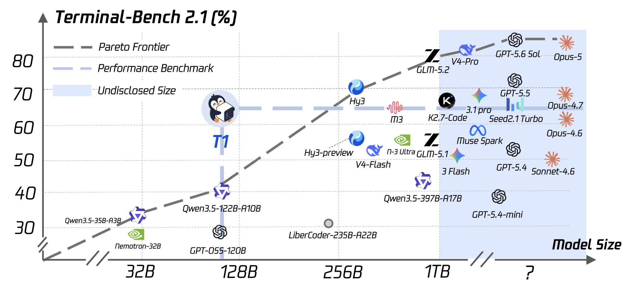
图 1|同一 harness 下的规模—性能定位。横轴为模型规模,纵轴为 Terminal-Bench 2.1 解决率。 在 122B 这一档,T1 高于 GPT-5.4(54.8)、DeepSeek-V4-Flash(56.9),也高于 Claude Opus 4.6(63.8), 并逼近生产级的 Claude Opus 4.7(66.1),是同规模区间里最好的模型。
Figure 1 | Performance against frontier models under the Harbor / Terminus-2 harness. Model size on the horizontal axis, Terminal-Bench 2.1 resolved rate on the vertical axis. At the 122B scale, T1 sits above GPT-5.4 (54.8), DeepSeek-V4-Flash (56.9) and even Claude Opus 4.6 (63.8), approaches the production-grade Claude Opus 4.7 (66.1), and is the best model in its size band.
这份报告是什么What this report is

它是一份系统报告,不是算法论文。四个贡献:(1) 超大 MoE Agent RL 的稳定化栈的代码级记录 (TITO、R³、critic 调度及周边容错机制);(2) 稠密过程奖励的设计与实测行为,包括两个失败的奖励变体及原因; (3) 在 95 GiB 显存的 GPU 上把一对 122B 的 PPO actor–critic 养活数天所需的基础设施; (4) 一份坦诚的失败记录——我们觉得它至少和成功一样有教益。

This is a systems report, not an algorithms paper. Its contributions are (1) a code-level account of the stabilization stack for very large MoE agent RL (TITO, R³, critic schedule, and the surrounding failure-handling machinery); (2) the design and measured behavior of the dense process reward, including two reward variants that failed and why; (3) the infrastructure required to fit and keep alive a PPO actor–critic pair of 122B models on 95 GiB GPUs for days; and (4) a candid record of the failures encountered, which we found at least as instructive as the successes.

02模型、任务与数据Model, task and data

模型Model

底座是一个 48 层的混合注意力 MoE decoder:hidden size 3072,32 个注意力头配 2 个 KV group(GQA), gated attention output、RMSNorm、部分 RoPE,词表 248,320。注意力按 3:1 的模式交替 ——三层 GatedDeltaNet 线性注意力接一层全注意力。每一层都带 MoE FFN:256 个专家, fp32 下 softmax top-8 路由,外加一个门控共享专家。总参数 121.4B,其中 116.0B 是专家权重, 每 token 激活约 10B。RL 阶段关闭 MoE 的辅助负载均衡损失。

起点有两个 checkpoint:base 模型(Terminal-Bench 2.1 上 43.8%)和一个称为 RST 的 SFT checkpoint(49.4%)。 本报告的主力实验都从 RST 出发。

The backbone is a 48-layer hybrid-attention MoE decoder: hidden size 3072, 32 attention heads with 2 KV groups (GQA), gated attention output, RMSNorm, partial RoPE, vocabulary 248,320. Attention alternates in a 3:1 pattern — three GatedDeltaNet linear-attention layers, then one full-attention layer. Every layer carries an MoE FFN: 256 experts, softmax top-8 routing in fp32, plus a gated shared expert. Total parameters 121.4B, of which 116.0B are expert weights; active parameters per token are ~10B. During RL the MoE auxiliary load-balancing loss is disabled.

Two starting checkpoints appear: the base model (43.8% on Terminal-Bench 2.1) and an SFT checkpoint referred to as RST (49.4%). The main campaigns of this report all start from RST.

任务与 Agent harnessTask and agent harness

Agent 是 Terminus-2(经由 Harbor):一个 JSON 工具调用循环,assistant 每轮发 shell 命令,tool 每轮返回终端输出。 生产配置的单次试验上限为:最多 60 轮、Agent 墙钟 3600 秒、验证器墙钟 900 秒、chat template 里关闭 thinking, 以及主动上下文压缩(Agent 自己总结历史)。沙箱是 Daytona 云容器(10 GiB 磁盘),每次试验创建后销毁。

一个任务就是一个自包含目录:task.toml 固定元数据与限额,instruction.md 描述一个长程终端任务 (比如:在两百个 commit 里做 bisect、修掉缺陷、重新构建到指定路径、并证明它成立), environment/ 放基础镜像和资源上限,tests/ 放验证器,solution/ 放 Agent 永远看不到的参考解。 验证器是承重结构:它跑 pytest --ctrf 并吐出逐测试的通过/失败记录, 于是奖励是被执行出来的而不是被建模出来的,且分辨率细到单条断言而非每轨迹 1 bit。

The agent is Terminus-2 (via Harbor): a JSON-tool-call loop in which each assistant turn issues shell commands and each tool turn returns terminal output. Per-trial limits in the production configuration: at most 60 turns, agent wall-clock 3600 s, verifier wall-clock 900 s, thinking disabled in the chat template, and proactive context compaction (the agent summarizes its own history). Sandboxes are Daytona cloud containers (10 GiB disk), created and destroyed per trial.

A task is a self-contained directory: task.toml fixes metadata and per-trial limits, instruction.md states a long-horizon terminal mission (bisect two hundred commits, repair the defect, rebuild to a named path, and prove it), environment/ carries the base image and resource caps, tests/ holds the verifier, and solution/ a reference solution the agent never sees. The verifier is the load-bearing part: it runs pytest --ctrf and emits a per-test pass/fail record, so the reward is executed rather than modelled, and its resolution is per assertion rather than one bit per trajectory.

训练数据池Training data pools

Category composition of Strategy-15k
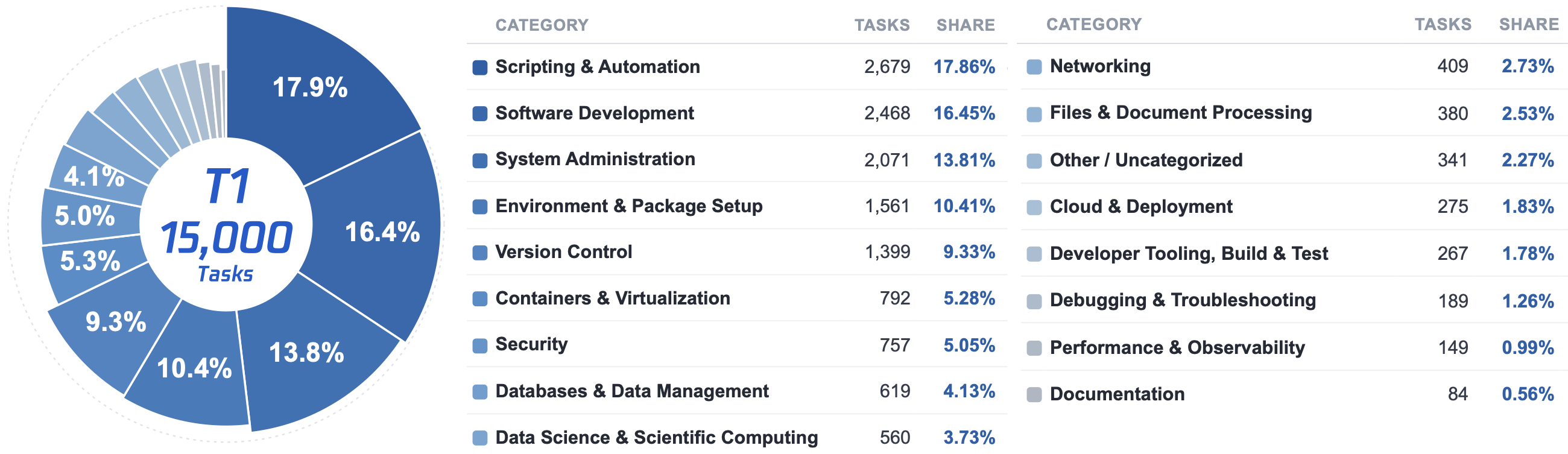
图 2|Strategy-15k 的类别构成。15,000 个任务归并到 17 个类别(原始 47 个标签)。 角度精确编码占比,半径是基于排名的幂次刻度(为了让小切片仍可见,因此与占比成正比)。 数据池明显集中在命令行工程:脚本与自动化 17.9%、软件开发 16.5%、系统管理 13.8%、 环境与包配置 10.4%、版本控制 9.3%,前五类占了 67.9%; 而数据科学(3.7%)、调试(1.3%)、性能优化(1.0%)很薄——这个偏斜正好预示了残余失败会落在哪里。
Figure 2 | Category composition of Strategy-15k. All 15,000 tasks are counted once across 17 merged categories (from 47 raw labels); angle encodes share exactly, while radius is a rank-based power scale chosen to keep small slices visible and is therefore not proportional to share. The pool is concentrated in command-line engineering work: scripting and automation (17.9%), software development (16.5%), system administration (13.8%), environment and package setup (10.4%) and version control (9.3%) make up two-thirds of the pool, while data science (3.7%), debugging (1.3%) and performance work (1.0%) are thin — a skew predicting where residual failures land.
The eight audit dimensions and their weights
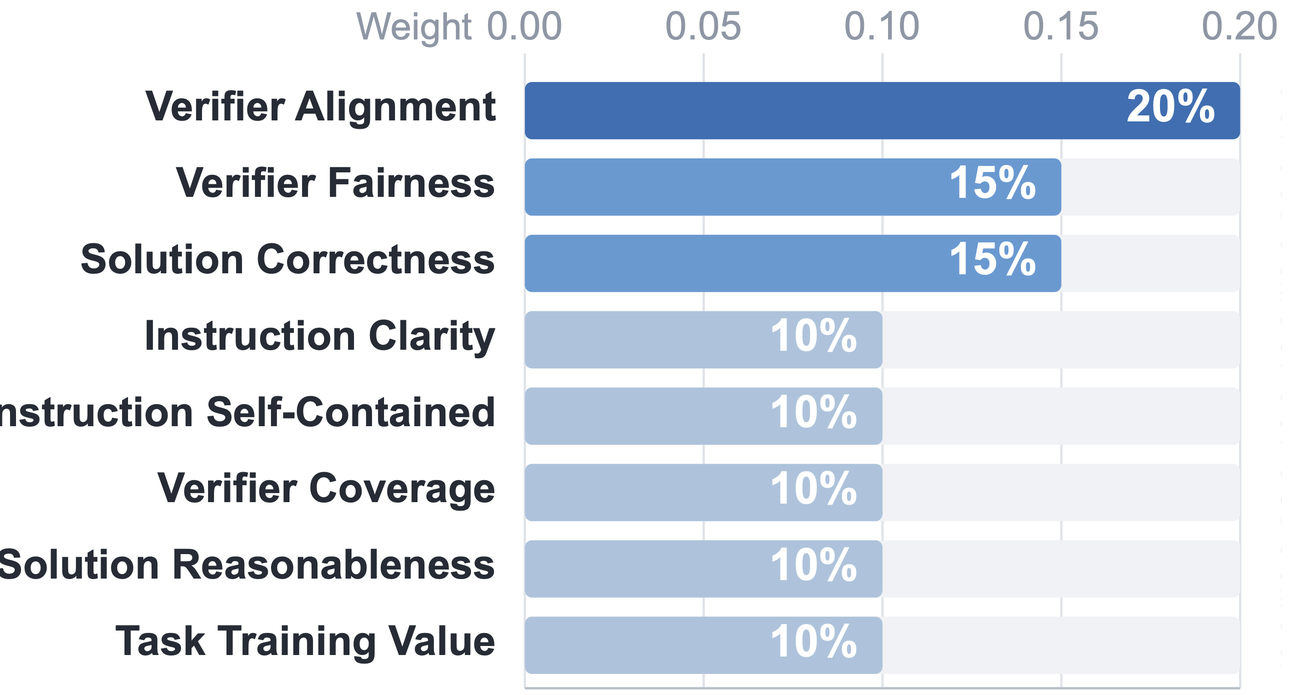
图 3|数据审计的八个维度及其权重(合计 1.00)。 按面归并:指令 40%、验证器 25%、解法 25%、任务价值 10%。 其中「指令 / 验证器一致性」单项权重最高(20%),因为公开指令与 tests/ 实际强制内容不一致 ——即隐藏需求——会让一个任务作为 RL 信号彻底失效:Agent 因为一条它从未被告知的判据而受罚。 筛选分五个阶段、跨 15 轮改写完成,包含可执行校验(参考解必须真的在容器里通过自己的验证器)、 语义审查(5,902 通过 / 3,251 边界 / 5,847 拒绝)、只改指令不动测试的修复(6,875 个任务)以及一次对抗式复审。
Figure 3 | The eight audit dimensions and their weights, summing to 1.00. Rolled up by facet: instruction 40%, verifier 25%, solution 25%, task value 10%. Instruction / verifier alignment carries the largest single weight (20%) because a mismatch between the public instruction and what tests/ enforces — a hidden requirement — makes a task unusable as an RL signal: the agent is punished for failing a criterion it was never shown. Selection ran in five stages over 15 rewrite rounds, including executable validation (the reference solution genuinely passes its verifier in-container), a semantic pass (5,902 accept / 3,251 borderline / 5,847 reject), instruction-only repair (6,875 tasks, leaving tests/ untouched), and an adversarial re-audit.

评测协议与算力Evaluation protocol and compute

留出评测是 Terminal-Bench 2.1 的 89 个终端任务,指标为解决比例,走与训练完全相同的 harness 和沙箱后端, 每任务 3 次尝试,温度 1.0、top-p 0.95、top-k 20。 评测总超时很关键:早期 3600 秒的墙会静默取消约 14 个慢任务,把 base 模型的测量分从约 0.43 拖到 0.371; 生产配置把它抬到 10,800 秒,并加了一道验收门——attempt 覆盖率不等于 1.0 就拒绝开始训练。

生产稠密奖励实验用 128 张 GPU:64 张训练(TP2 × PP4 × CP4 ⇒ DP2,EP16,每流水段 12 层) + 64 张推理(8 个独立 SGLang 引擎,各 TP8),每步 512 条轨迹,约 57 分钟一步。 早期二值奖励实验用 88 张卡,batch 256 时约 33 分钟一步。

Held-out evaluation is Terminal-Bench 2.1: 89 terminal tasks, scored as the fraction resolved, run through the same harness and sandbox backend as training, with 3 attempts per task at temperature 1.0, top-p 0.95, top-k 20. The evaluation-total timeout matters: an early 3600 s wall silently cancelled ~14 slow tasks and dragged the base model's measured score from ~0.43 to 0.371; production configs raise it to 10,800 s. A baseline-eval acceptance gate refuses to start training unless attempt coverage is exactly 1.0.

The production dense-reward run uses 128 GPUs: 64 training GPUs (TP2 × PP4 × CP4 ⇒ DP2, EP16, 12 layers per pipeline stage) and 64 inference GPUs (8 independent SGLang engines at TP8), batch 512 trajectories per step, ~57 min/step. Earlier binary-reward runs used 88 GPUs, measured at ~33 min/step at batch 256.

03训练系统Training system

我们构建在 slime v0.3.0 之上,它把 Megatron 训练后端和 SGLang 推理引擎放进同一个 Ray 应用。 学习和 rollout 占用互不重叠的 GPU,并且流水线深度为一步:第 t 步在训练时, 第 t+1 步的 batch 已经在生成了。上游提供了 PPO critic 脚手架、路由记录/回放核心、 token 级动态批处理和按角色的优化器配置;我们的终端 Agent 集成是增量式的,通过公开扩展点挂载而非 fork ——核心改动约 1k 行,插件约 7.8k 行。

We build on slime v0.3.0, which places a Megatron training backend and SGLang inference engines under one Ray application. Learning and rollout occupy disjoint GPUs and are pipelined one step deep: while step t trains, the batch for step t+1 is already generating. Upstream supplies the PPO critic scaffolding, the routing record/replay core, token-level dynamic batching, and per-role optimizer configuration; our terminal-agent integration is additive, attached through public extension points rather than a fork — ~1k lines of core delta, ~7.8k of plugin.

The T1 training pipeline
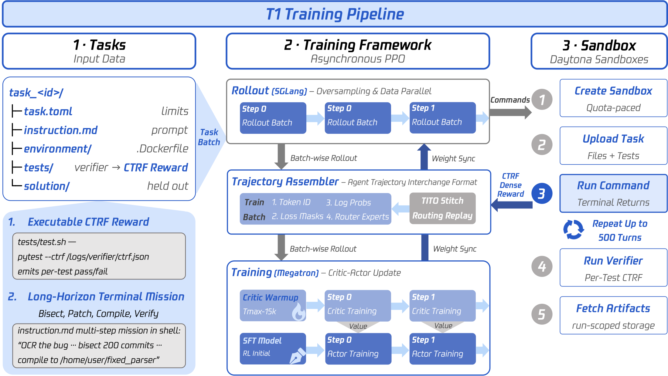
图 4|T1 训练流水线。 左:每个任务是一个自包含目录——元数据、长程指令、带资源限制的环境镜像、留出验证器、参考解, 其测试吐出逐测试 CTRF 记录,让奖励可执行而非被建模。 中:SGLang 在过采样下服务行为策略;轨迹装配器把交互日志规范化成 TITO 拼接的训练样本, 连带路由行和 CTRF 稠密奖励;Megatron 先更新 critic 再更新 actor,然后把权重同步回去。 右:Daytona 沙箱被创建、加载、逐轮驱动、验证、回收。rollout 与训练在不重叠的 GPU 上并发。
Figure 4 | The T1 training pipeline. Left: each task is a self-contained directory — metadata, a long-horizon instruction, an environment image with resource limits, a held-out verifier, and a reference solution — whose tests emit a per-test CTRF record, making the reward executable rather than modelled. Middle: SGLang serves the behaviour policy under oversampling; the trajectory assembler normalizes interaction logs into TITO-stitched training samples with routing rows and the CTRF dense reward; Megatron updates critic then actor and synchronizes weights back. Right: Daytona sandboxes are created, loaded, driven turn by turn, verified, and reclaimed. Rollout and training run concurrently on disjoint GPUs.

Rollout 与轨迹装配Rollout and trajectory assembly

从 SFT checkpoint 出发,SGLang 向大量并发试验提供行为策略。调度器会过采样: 启动比 batch 所需更多的试验,接受最先完成的 B 个,取消长尾——这是在一个完成时间重尾的环境里 约束单步时长的关键手段。Agent 与引擎交换的是 token id 而不是文本, 并拿回采样到的 id、逐 token 的对数概率和逐 token 的专家路由。

完成的试验进入轨迹装配器:被采样的 assistant token 保留其 id、对数概率和单位损失掩码; 工具观测和模板胶水以掩码形式进入。路由行与 token 流严格同步推进,每个试验的 CTRF 记录成为它的稠密奖励。 最终发出的训练 batch 把 token id、损失掩码、推理侧对数概率和被路由的专家放在一起携带 ——任何触碰逐 token 数据的环节都必须用相同的偏移量变换这四者,这是整条流水线的中心不变式。

Starting from the SFT checkpoint, SGLang serves the behaviour policy to many concurrent trials. The scheduler oversamples: it launches more trials than the batch requires, accepts the first B to complete, and cancels the straggler tail, which is what bounds step time against an environment whose completion times are heavy-tailed. The agent exchanges token ids rather than text with the engines and receives sampled ids, per-token log-probabilities, and per-token expert routing.

Completed trials enter the trajectory assembler: sampled assistant tokens keep their ids, log-probabilities and a unit loss mask; tool observations and template glue enter masked. Routing rows advance in lock-step with the token stream, and each trial's CTRF record becomes its dense reward. The emitted train batch carries token ids, loss masks, inference log-probabilities and routed experts together — every stage that touches per-token data transforms all four by the same offsets, which is the pipeline's central invariant.

Critic 与 actor 的更新次序Critic and actor updates

Megatron 消费这个 batch。任何策略移动之前先有一段简短的 critic 预热; 之后每一步都先跑 critic:它的更新前价值同时喂给优势估计器和它自己的裁剪价值损失, 并以 actor 的 30 倍学习率训练,因为它的目标是一个监督回归。 随后 actor 在行为快照下重算旧的对数概率,走一步裁剪代理目标。 奖励落在最后一个响应 token 上,由 GAE 在整个长程上做信用分配;由于每任务只采 1 条样本, 没有组基线,critic 是唯一的基线。又因为 actor 和 critic 同样大小、靠强制 offload 共享 GPU, 这个次序也是显存唯一允许的次序。

Megatron consumes the batch. A brief critic warm-up precedes any policy movement, after which each step runs the critic first: its pre-update values feed both the advantage estimator and its own clipped value loss, and it trains at 30× the actor's learning rate because its target is a supervised regression. The actor then recomputes old log-probabilities under the behaviour snapshot and takes one clipped-surrogate step. The reward lands on the final response token and GAE performs credit assignment across the horizon; with one sample per task there is no group baseline, so the critic is the only baseline. Because actor and critic are the same size and share GPUs by forced offload, this ordering is also the only one memory permits.

权重同步Weight synchronization

更新后的权重每步向所有引擎发布一次,发布前先让生成静默,保证没有请求跨越两个策略版本。 行为快照在同一个 barrier 内轮换,于是重要性比率的分母始终是真正采样了这个 batch 的那个策略: 流水线带来的一步滞后是恰好一步的普通 off-policy,而不是未建模的偏差。 这样 rollout 就藏在训练之下,单步时长是 max(rollout, training) 而不是二者之和。

Updated weights are published to every engine once per step, with generation quiesced first so no request spans two policy versions. The behaviour snapshot rotates inside the same barrier, so the importance ratio's denominator remains the policy that actually sampled the batch: the one-step lag introduced by pipelining is ordinary off-policyness of exactly one step rather than unmodeled bias. Rollout thus hides under training, making step time max(rollout, training) instead of their sum.

04PPO

PPO 核心刻意做得很朴素。裁剪比率 ε = 0.2(对称),KL 惩罚与 KL 损失关闭, 熵奖励关闭(仍以无梯度方式记录),MoE 辅助负载均衡损失关闭。 优势估计器为 ppo(critic + GAE),γ = 1、λ = 1,价值裁剪 0.2, 锚定 critic 的更新前价值。每个 prompt 采 1 条样本(因此无组归一化、无组基线), batch 512 条轨迹,token 预算墙 84k(二值奖励实验为 64k)。 优化器 Adam(0.9, 0.98)、weight decay 0.1、恒定学习率, actor 1.0 × 10⁻⁶、critic 1.5 × 10⁻⁵(30× 差距),critic 热加载后再做 2 步 critic-only 重校准。 精度为 bf16 权重 + fp32 梯度累积,路由打分 fp32 softmax,不使用 fp8。 PPO 比率的分母是训练侧重算的旧对数概率,TIS 修正只记录、不施加到损失。 3 个 epoch × 15,000 任务 ÷ batch 512 = 90 步。

The PPO core is deliberately spare. Clip ratio ε = 0.2 (symmetric); KL penalty and KL loss off; entropy bonus off (still logged no-grad); MoE auxiliary load-balancing loss off. The advantage estimator is ppo (critic + GAE) with γ = 1, λ = 1, and a value clip of 0.2 anchored to the critic's pre-update values. Each prompt is sampled once (hence no group normalization and no group baseline), the batch is 512 trajectories, and the token-budget wall is 84k (64k for the binary-reward runs). The optimizer is Adam(0.9, 0.98) with weight decay 0.1 and a constant learning rate, at 1.0 × 10⁻⁶ for the actor and 1.5 × 10⁻⁵ for the critic (a 30× gap), with the critic warm-loaded and given 2 critic-only re-calibration steps. Precision is bf16 weights with fp32 gradient accumulation, router scores in fp32 softmax, no fp8. The denominator of the PPO ratio is the training-side recomputed old log-probabilities, and TIS correction is recorded but not applied to the loss. Three epochs over 15,000 tasks at batch 512 is 90 steps.

05让 MoE 的 RL 训练稳下来Stabilizing MoE RL training

PPO 的重要性比率隐含一个前提:训练器评估的,必须等于采样器在同一版本上真正实现的。 在这个设定下它以两种方式失效,而且这两种失效相互独立——修好一个不会碰到另一个。

PPO's importance ratio rests on one requirement: what the trainer evaluates must equal what the sampler realized at the same policy version. In this setting it fails in two ways, and the two are independent — enforcing one leaves the other's failure mode untouched.

稠密模型根本不会犯第二种错,短程任务会稀释第一种错。但一个发出 20–60 轮轨迹的 122B MoE 会在约 10⁴ 个 token 上 同时犯这两种错,而误差是乘性累积的:缓解前逐 token 的平均对数概率偏差 0.021, 在约 3 × 10⁴ 个 token 上会产生一个 PPO 裁剪无法与真实策略移动区分开的比率误差。

Dense models cannot violate the second identity at all, and short horizons attenuate the first. But a 122B MoE emitting 20–60-turn trajectories violates both across ~10⁴ tokens, and the error compounds multiplicatively: a mean per-token log-probability discrepancy of 0.021 before mitigation, over ~3 × 10⁴ tokens, produces a ratio error the PPO clip cannot separate from genuine policy movement.

TITO:token 进,token 出TITO: token-in, token-out

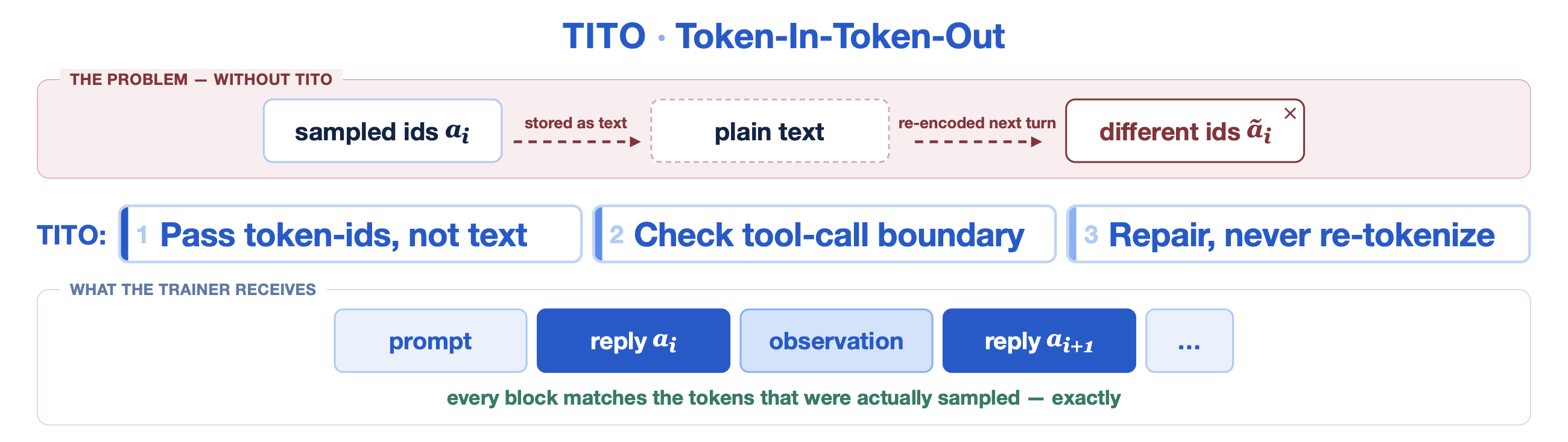
TITO 用构造的方式强制 token 保真:训练器消费的正是引擎发出的那些 id,反之亦然。 在我们控制两端的地方,「解码再编码」被直接消除;在 harness 强制它发生的地方,则被检测并修复。 Harbor 后端双向传输 token id,因此编码每轮只做一次,而不是每次重放历史都做一次。 轮次之间,装配器依次尝试四种越来越弱的前缀关系:strict(严格前缀,这就是精确的 TITO)、 normalized(在一个 97 × 17 的有限网格上做有界修复,因此是可审计的而非启发式的)、 retokenized(token 层面全面失配时退化到文本空间的相等性,靠生成时的偏移映射定位区间)、 以及 split(都不成立就切成共享 group id 的新 chunk)。 关键是:harness 重新分词后的那份拷贝永远不会进入训练流,进入的始终是被采样的原始 id。

TITO enforces token fidelity constructively: the trainer consumes exactly the ids the engine emitted, and vice versa. Where we control both endpoints, encode-of-decode is eliminated; where the harness forces it, it is detected and repaired. The Harbor backend transmits token ids in both directions, so encoding happens once per turn rather than once per history replay. Between turns the assembler tests four progressively weaker prefix relations: strict (exact prefix — this is exact TITO), normalized (a bounded repair over a finite 97 × 17 grid, which makes it auditable rather than heuristic), retokenized (when token matching fails everywhere, fall back to equality in text space and locate the span by a generation-time offset map), and split (neither holds → a new chunk sharing the same group id). The key property: the harness's re-tokenized copy never enters the training stream; the sampled ids do.

TITO stitching
图 5|TITO 拼接,画的是四种情况里最难的 retokenized。 harness 重新分词的拷贝不进入训练流,被采样的 id 才进入,因此每一个承载损失的位置都严格满足 token 保真。 观测和模板胶水以掩码上下文的形式进入(掩码 0、对数概率 0)。在 strict 情况下,中间那条泳道与顶部逐 token 相同。
Figure 5 | TITO stitching, drawn for the retokenized case — the hardest of the four. The harness's re-tokenized copy never enters the training stream; the sampled ids do, so every loss-bearing position satisfies token fidelity exactly. Observations and template glue enter as masked context (mask 0, log-prob 0). Under strict, the middle lane is token-identical to the top one.

这里的保证是单边但锐利的:掩码为 1(即承载损失)的位置,其 token 必然与采样时逐位相同; 可能有偏差的只是后续轮次的条件化上下文。一次离线审计(1,402 个样本、2725 万条路由行)给出了实测数字: 97.39% 的位置逐位对齐,2.61% 属于重新分词或占位集合, 而落在损失区内的漂移比例是 0.0000%——漂移集合与损失区完全不相交。 值得一提的是,轨迹级的标志位是所有轮次「均为 strict」的合取,因此在约 99.9% 的轨迹上都读作 False; 只有逐 token 的统计才看得出真正要紧的那部分漂移其实是零。

The guarantee is one-sided but sharp: at every position whose mask is 1 (i.e. loss-bearing), the token is bit-identical to what was sampled; what can deviate is only the conditioning context of later turns. An offline audit (1,402 samples, 27.25M routing rows) gives the measured numbers: 97.39% of positions exactly aligned, 2.61% in the re-tokenized or placeholder sets, and 0.0000% drift inside the loss region — the drift set is disjoint from the loss region. Note that the trajectory-level flag is a conjunction over all turns being strict, and so reads False on ~99.9% of trajectories; only per-token accounting reveals that the drift that matters is zero.

R³:rollout 路由回放R³: rollout routing replay

R³ 同样用构造的方式强制路由保真:记录推理选择了哪些专家,再约束训练前向复用它们。 打过补丁的 SGLang 逐 MoE 层记录 top-k 索引,以 base64 的 int32 张量返回; 所有 48 层全部保存,不压缩、不抽样、不做门控,代价是每 token 1536 字节 ——一条 33k token 的轨迹约 48 MiB。路由行与 token 走完全相同的拼接逻辑, 保证第 j 行索引的就是第 j 个 token。在被修复过的边界上,某一行可能不属于任何一轮的记录, 此时构造器只在不可能影响任何梯度的位置替换为邻居行,否则直接报错。 路由缺失是硬错误,rollout 会中止而不是丢样本——丢样本等于把 batch 条件化在「记录成功」这个事件上,会引入偏差。

R³ enforces routing fidelity by construction: record the expert sets inference selected, and constrain the training forward to reuse them. A patched SGLang records top-k indices per MoE layer and returns a base64 int32 tensor; all 48 layers are stored with no compression, subsampling or gating, at a cost of 1536 bytes per token — about 48 MiB for a 33k-token trajectory. Routing rows ride exactly the same stitching as tokens, so row j indexes token j. At repaired boundaries a row may exist in no turn's capture; the builder then substitutes a neighbour row only where no gradient can be affected, and otherwise raises. Absent routing is a hard error and the rollout aborts rather than dropping the sample — dropping would condition the batch on the event "capture succeeded" and bias it.

注入这一侧,我们包装而非 fork Megatron 的 router:替换的是「选择」算子,「门控」仍走实时打分。 专家索引来自记录(无梯度),门控权重从当前参数的实时打分里 gather(梯度照常流动)。 用查表替代 top-k 消除了那个让微小数值差异变得要紧的不连续性, 而从实时打分读门控又让 router 保持可训练。每次前向之前,路由张量都会被施加与 token 流完全相同的 序列并行、padding、上下文并行 zig-zag 切分等变换——任何别的组合顺序都会错位并静默回放错误的专家, 所以每个样本都断言了行数与 token 数的关系。critic 从不回放:它的回归目标不需要对采样器的行为保真。

On the injection side we wrap rather than fork Megatron's router: the selection operator is substituted while gating stays on live scores. Expert indices come from the record (no gradient); gating weights are gathered from the live scores of the current parameters (gradient flows). Replacing top-k by a table lookup removes the discontinuity that made tiny numeric differences consequential, while reading gating from live scores keeps the router trainable. Before each pass, the routing tensor is put through exactly the token pipeline's transformations — sequence parallelism, padding, the context-parallel zig-zag slice — because any other composition would misalign rows and silently replay wrong experts, which is why the row-count relation is asserted per sample. The critic never replays: its regression target needs no behavioural fidelity to the sampler.

Critic 侧的稳定性Critic-side stability

这里的 PPO 用一个独立、全尺寸的 critic:第二个 122B 模型,把 LM head 换成最后一个流水段上的标量价值头。 它与 actor 共享同一个 placement group(不额外占卡),slime 强制训练侧 offload,让两个 122B 模型分时复用同一批 GPU ——每一个单独都必须塞进 95 GiB,这个约束直接驱动了后面的显存工程。

PPO here uses a separate, full-size critic: a second 122B model whose LM head is a scalar value head on the last pipeline stage. It shares the actor's placement group — no extra GPUs — and slime forces training-side offload so the two 122B models time-multiplex the same GPUs. Each alone must fit in 95 GiB, which is the constraint that drives the memory engineering below.

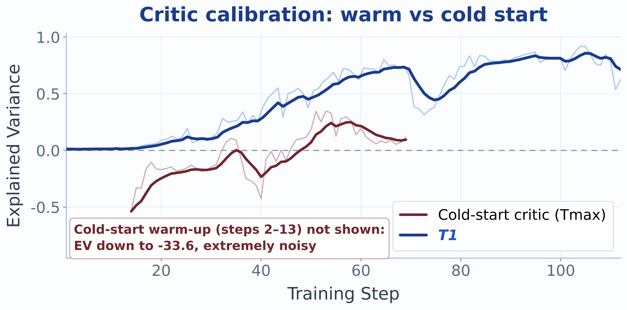
解释方差(EV)是这里最重要的健康指标:它是价值函数所解释的回报方差比例。 EV = 0 意味着 critic 不比预测 batch 均值更好;关键在于这个量下无界, EV < 0 意味着减去价值函数是在给优势增加方差而不是减少方差。 冷启动时 EV 从 −33.6 开始——新初始化的价值头的残差携带了约 34 倍于回报的方差 ——那次实验大约用前一半时间在偿还这个赤字。热加载直接消除了它: 稠密奖励实验从 0 附近开始,最终稳定在 0.71–0.86。这也解释了为什么 2 步 critic-only 就够, 而冷启动需要几十步:优势从第一次更新起就是方差被降低过的,而不是在前三分之一训练里被放大的。

Explained variance (EV) is the health metric that matters here: the fraction of return variance the value function accounts for. EV = 0 means the critic is no better than predicting the batch mean; crucially the quantity is unbounded below, and EV < 0 means subtracting the value function adds variance to the advantage instead of removing it. Cold-started, EV begins at −33.6 — the fresh value head's residuals carry ~34× the variance of the returns — and roughly the first half of that campaign pays down the deficit. Warm-loading removes it outright: the dense-reward run starts near 0 and settles at 0.71–0.86. This is why 2 critic-only steps suffice where a cold start needs tens: advantages are variance-reduced from the first update rather than variance-inflated for the first third of training.

Critic explained variance, warm versus cold start
图 6|Critic 解释方差,热启动对比冷启动。 蓝色(T1):生产稠密奖励实验(Strategy-15k)的热启动 critic。 酒红:TMax 实验的冷启动 critic,也正是蓝色实验所加载的那个 checkpoint。 浅线为逐步值,粗线为 EMA(α = 0.25),虚线标出 EV = 0。 冷启动从 EV = −33.6 开始(超出坐标范围),在 58 个记录步里有 30 步为负; 热启动实验从未转负,并稳定在 0.71–0.86。
Figure 6 | Critic explained variance, warm versus cold start. Blue (T1): the warm-started critic of the production dense-reward run (Strategy-15k). Wine red: the cold-started critic of the TMax campaign, whose checkpoint the blue run loads. Faint lines are per-step values, bold lines an EMA (α = 0.25); the dashed rule marks EV = 0. The cold start opens at EV = −33.6 (off scale) and is negative for 30 of 58 logged steps; the warm-started run never goes negative and plateaus at 0.71–0.86.

实测效果Measured effect

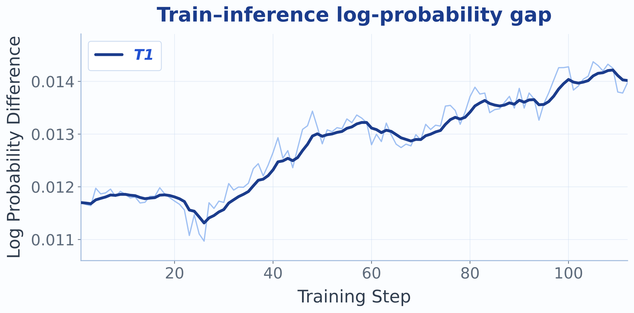
两个机制合起来把训推对数概率差距从 0.021 降到 0.013, 并且在整个 112 步里稳定保持在 0.0110–0.0144 这个很窄的带内。 残余的 0.013 非零是符合预期的:R³ 对齐的是专家选择而非 kernel 数值, 而且 reference 和 critic 的前向按设计自由路由。 同样值得说明的是,这个指标缓慢上飘不是回退:它度量的是训练策略与生成该 batch 的权重之间的距离, 策略正当地进步时它本来就会变大。

Together the two mechanisms reduce the train–inference log-probability gap from 0.021 to 0.013, holding a narrow 0.0110–0.0144 band for all 112 steps. That the residual 0.013 is nonzero is expected: R³ aligns expert selection but not kernel numerics, and the reference and critic paths route freely by design. Equally worth stating: this metric drifting slowly upward is not a regression — it measures the distance between the training policy and the weights that generated the batch, which grows as the policy legitimately improves.

Train-inference log-probability gap
图 7|训推对数概率差距。:生产稠密奖励实验的逐步序列,来自一个只做记录的失配钩子; 浅线为逐步值,粗线为 EMA(α = 0.25)。:同一个 122B 栈上,开启与关闭这两个机制时的平均差距 (0.013 对 0.021)。顺带一个坑:内置指标按 micro-batch 数而非掩码和归一化, 在 micro batch size 为 1 时会把它放大约 1000 倍,我们的钩子重新推导了正确的归约方式。
Figure 7 | Train–inference log-probability gap. Left: per-step series over the production dense-reward run, from a record-only mismatch hook; faint line is the per-step value, bold line an EMA (α = 0.25). Right: mean gap on the same 122B stack with and without the two mechanisms (0.013 vs 0.021). One trap worth noting: the built-in metric normalizes by micro-batch count rather than by the mask sum, inflating it ~1000× at micro-batch size 1; our hook re-derives the correct reduction.
三个反直觉的系统结论Three counter-intuitive systems findings

① RL 期间不加任何 router 辅助损失。负载均衡的压力会和 R³ 打架 (我们要求 router 复现 rollout 的选择,而不是重新均衡),并且引入一个与奖励无关的梯度。

② 超长样本无法用 token 预算限制住。slime 的 first-fit 打包会把超长样本 单独放进它自己的 bin 且保持全长,所以一条 40k token 的轨迹会自成一个 micro-batch, 与「每 GPU 最大 token 数」这个旋钮无关。所有想用那个旋钮修长序列 OOM 的尝试都是构造上注定失败的; 真正的杠杆是序列墙和上下文并行。

③ Triton 冷编译风暴看起来完全像 NCCL 挂死。变长轨迹 × 动态批处理每步会产生几十种 padding 形状, 每种都要 JIT 编译 GatedDeltaNet kernel 若干分钟。某次一个 rank 卡在 30 分钟以上的编译里, 它的 15 个专家并行同伴在 MoE all-to-all 上等待,最后 watchdog 杀掉的是那些同伴。 解法是更粗的 padding 粒度、节点本地的持久 Triton 缓存、120 分钟的 NCCL 组超时和超时即 dump 的 flight recorder。

① No auxiliary router losses during RL. Load-balancing pressure fights R³ (the router is asked to reproduce rollout choices, not re-balance) and adds a non-reward gradient.

② Oversized samples cannot be capped by token budgets. slime's first-fit packer places an oversized sample alone in its own bin at full length, so a 40k-token trajectory forms its own micro-batch regardless of the max-tokens-per-GPU knob. Every attempt to fix long-sequence OOMs with that knob failed by construction; the real levers are the sequence walls and context parallelism.

③ Triton cold-compile storms look exactly like NCCL hangs. Variable-length trajectories × dynamic batching produce dozens of padded shapes per step, each JIT-compiling GatedDeltaNet kernels for minutes. In one incident a single rank sat in a >30-min compile while its 15 expert-parallel peers waited in the MoE all-to-all; the watchdog killed the peers. Mitigations: coarser padding granularity, a persistent node-local Triton cache, 120-min NCCL group timeouts, and flight-recorder dumps on timeout.

06稠密奖励:CTRF 测试计数Dense reward: the CTRF test count

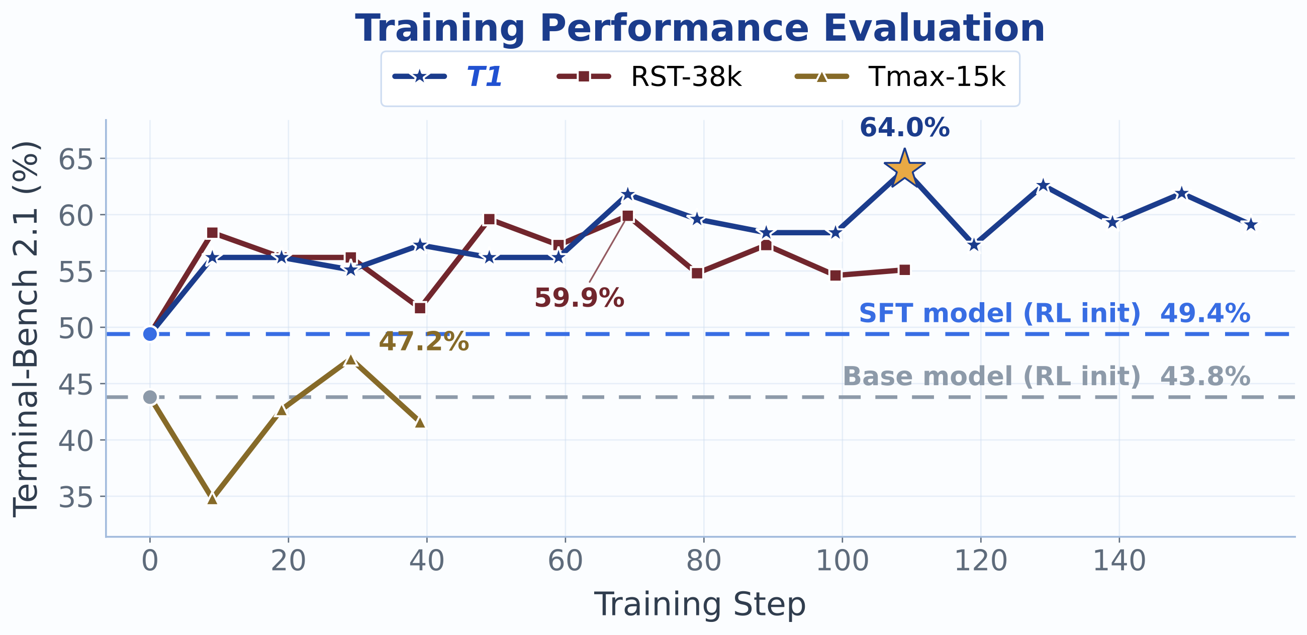
第一次 122B 实验在 TMax 上用朴素的二值「任务是否解决」奖励。它在 40 步内把 base 模型从 43.8% 推到 47.2%, 但始终没有超过 SFT 的 49.4%。两个结构性读解:数据池相对 RST 太容易(没有可学的头部空间), 而对那些验证器里本来就含有许多可独立检查的断言的任务来说, 「每条耗费数千沙箱秒的轨迹只给 1 bit」是一个极低的信号率。那次实验最终只留下一个用途 ——在便宜且稳定的数据上把 critic 预热好。

The first 122B campaign trained on TMax with the plain binary task-solved reward. It moved the base model from 43.8% to 47.2% within 40 steps, but never exceeded the SFT checkpoint's 49.4%. Two structural readings: the pool is too easy relative to RST (little headroom to learn), and one bit per multi-thousand-sandbox-second trajectory is a very low signal rate for tasks whose verifiers actually contain many individually checkable assertions. The campaign was retained for exactly one purpose — warming up the critic on cheap, stable data.

转折点是让奖励可执行且有分辨率。每个任务的 tests/test.sh 在沙箱里跑 pytest --ctrf,验证器因此吐出一份标准的 CTRF JSON,里面有逐测试的汇总。 rollout 之后,奖励钩子读回每个试验的 verifier/ctrf.json,计算:

The turning point was making the reward executable and resolved. Each task's tests/test.sh runs pytest --ctrf inside the sandbox, so the verifier emits a standard CTRF JSON with a per-test summary. After rollout, the reward hook reads each trial's verifier/ctrf.json back and computes:

r = # passed tests S , S = 20
通过测试的绝对数量,除以一个固定的全局尺度——明确不是通过率。
the absolute passed-test count on a fixed global scale — explicitly not the pass ratio.

两个设计决定值得展开:

Two design decisions are worth spelling out:

这里的「稠密」指的是奖励的取值分辨率(0、1/20、2/20 …),不是它的放置位置: 标量仍然只加在每个轨迹 chunk 的最后一个响应 token 上,由 critic + GAE 在 60 轮的长程上做时序信用分配。 没有势函数式 shaping,也没有逐轮奖励。PPO 下奖励原样流入 critic:不做组归一化, 也没有开启优势归一化。由于每任务只有 1 条样本,也没有组基线——critic 是唯一的基线, 所以它的校准处在关键路径上。

"Dense" here refers to the reward's value resolution (0, 1/20, 2/20, …), not its placement: the scalar still enters at the last response token of each trajectory chunk, and the critic + GAE performs temporal credit assignment across the 60-turn horizon. There is no potential-based shaping and no per-turn reward. Under PPO the rewards flow into the critic raw: no group normalization, and advantage normalization is not enabled. With one sample per task there is also no group baseline — the critic is the only baseline, which is why its calibration is on the critical path.

CTRF dense reward curve
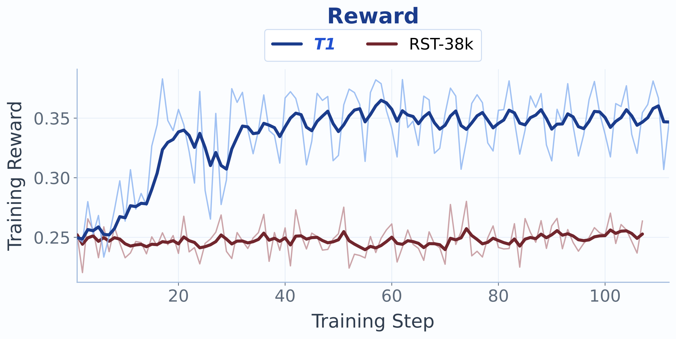
图 8|生产稠密奖励实验中的平均 rollout 奖励(原始值,未经任何归一化)。 浅线为逐步均值,粗线为 EMA(α = 0.25)。奖励在前 30 步从 0.250 升到约 0.345, 随后 80 步维持在 0.34–0.36 的带内,第 58 步附近峰值 0.365。 对照设计意图来读:S = 20 时均值约 0.35 对应每条轨迹约 7 个通过测试, 舒服地落在信号分辨率之内而不是被顶在任何一端——这恰恰是比率形式会通过封顶而摧毁的东西。 平台期不是停滞:留出基准在这段时间里仍在提升,说明模型是在重新分配它通过哪些测试, 而不是简单地多过几个。可见的高频振荡是 batch 512、每任务 1 样本下洗牌带来的批构成特征,不是不稳定 ——它的幅度(约 0.02)在整个实验里保持恒定。
Figure 8 | Mean rollout reward under the CTRF test-count reward over the production dense-reward run (raw values, before any normalization). Faint line: per-step mean; bold line: EMA (α = 0.25). Reward rises from 0.250 to ~0.345 in the first 30 steps and then holds a 0.34–0.36 band for the remaining 80, peaking at 0.365 near step 58. Read against the design choices: a mean of ~0.35 at S = 20 corresponds to roughly 7 passing tests per trajectory, comfortably inside the resolution of the signal rather than pinned at either end — precisely what the ratio formulation would have destroyed by capping every task at 1.0. The plateau is not stagnation: the held-out benchmark keeps improving through it, so the run is redistributing which tests it passes rather than simply passing more of them. The visible high-frequency oscillation is the batch-composition signature of shuffling at batch 512 with one sample per task, not an instability — its amplitude (~0.02) stays constant over the run.

两次失败的长度整形,和一个修好的版本Length shaping: two failures and a fix

我们实现过三个针对轨迹膨胀的长度整形变体,生产主实验一个都没用,但它们的历史很有教育意义:

Three optional variants shape the test-count reward against trajectory bloat; the production run uses none of them, but their histories are instructive:

洗牌是奖励设计的一部分Shuffling is part of the reward design

Strategy-15k 是按质量排名顺序物化在磁盘上的(第一个任务就是最好的那个)。 不洗牌的话,顺序游标会从最好扫到最差,每个 512 任务的 batch 都来自一个很窄的质量带 ——critic 看到的奖励分布会在一个 epoch 内单调漂移。因此我们对整池施加「种子 + epoch」的置换, 让每 batch 的奖励统计保持平稳。15,000 个任务、batch 512、3 个 epoch,正好是 90 步。

Strategy-15k is materialized in quality-rank order (the first task is the best one). Without shuffling, a sequential cursor would sweep best-to-worst and every 512-task batch would come from one narrow quality band — the reward distribution the critic sees would drift monotonically over the epoch. We therefore apply a seed+epoch permutation over the pool, keeping per-batch reward statistics stationary. Three epochs over 15,000 tasks at batch 512 is exactly 90 steps.

07结果Results

三个实验构成了完整的故事线:TMax 上的二值奖励(从 base 出发)早期能改进 base 模型 (43.8% → 第 29 步的 47.2%),但从未追上 SFT 的 49.4%,它留下的资产是那个训练好的 critic; RST-38k 上的稠密奖励(未过滤,从 RST 出发)立刻越过 SFT(第 9 步 0.584), 在 0.52–0.60 的带内振荡,峰值 0.599;而 Strategy-15k 上的稠密奖励(已过滤、从 RST 出发、critic 热加载) 是本报告的生产实验:前两个 epoch 稳在 0.55–0.57,第三个 epoch 向上突破 ——第 69 步 0.618,第 109 步的重复评测给出 0.596–0.635(最好 0.635 = 57/89)。 我们把第 69 步那次干净的单次评测作为主报数,并把第 109 步的分散度当作 n = 3、89 个任务下评测方差的诚实写照。

Three campaigns structure the story. Binary reward on TMax (from base) improves the base model early (43.8% → 47.2% at iteration 29) but never reaches the SFT checkpoint's 49.4%; its lasting contribution is the trained critic. Dense reward on RST-38k (unfiltered, from RST) jumps immediately above SFT (0.584 at iteration 9) and oscillates in the 0.52–0.60 band, peaking at 0.599. Dense reward on Strategy-15k (filtered, from RST, warm critic) is the production run of this report: it holds 0.55–0.57 for the first two epochs, then breaks upward in the third — 0.618 at iteration 69, and at iteration 109 repeated evaluations give 0.596–0.635 (best 0.635 = 57/89). We quote iteration 69's single clean evaluation as the headline and treat the iteration-109 spread as an honest picture of evaluation variance at n = 3 on 89 tasks.

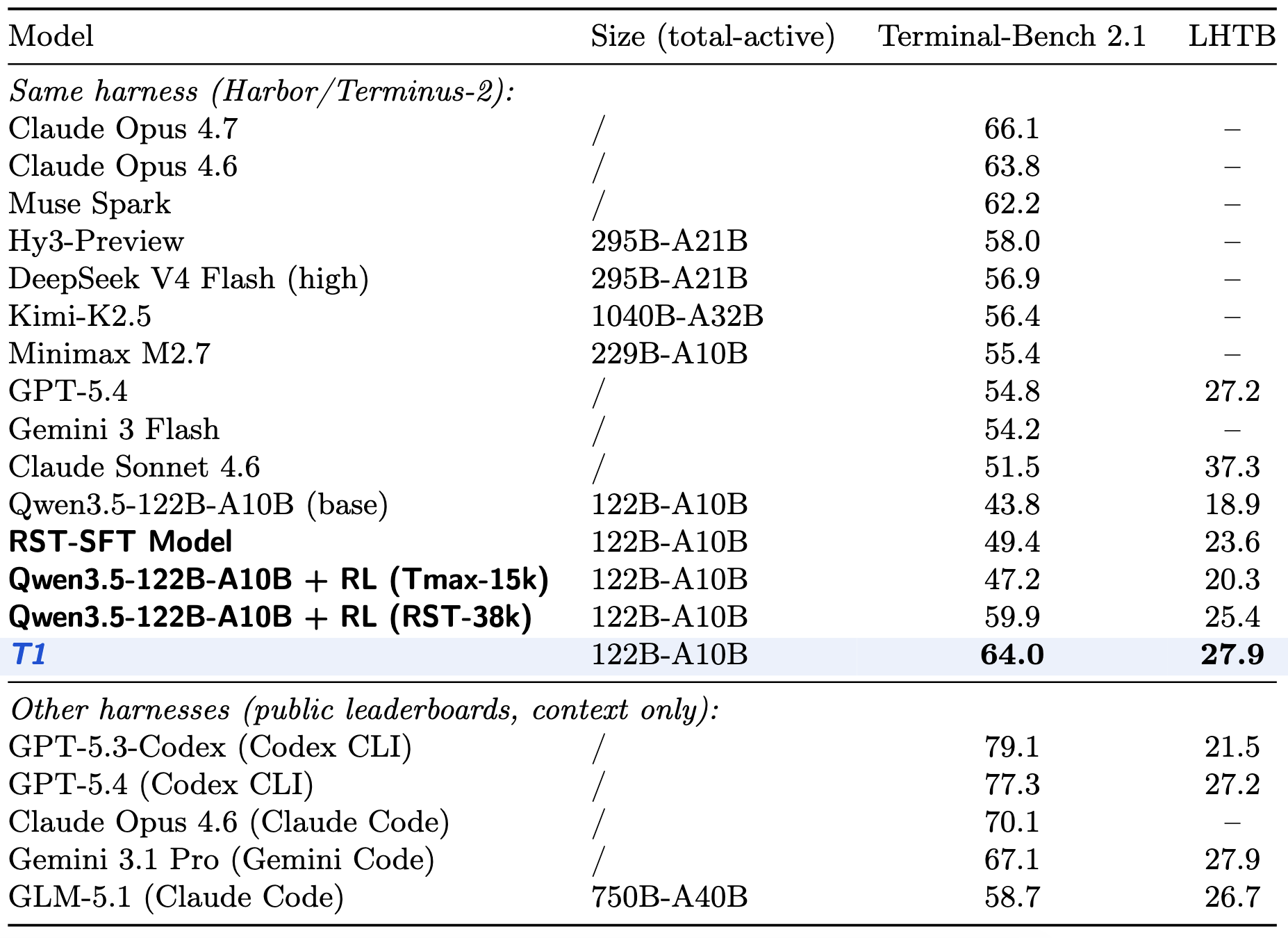
表 1|Terminal-Bench 2.1 对比。上半部分是与我们同一 Harbor / Terminus-2 harness 下评测的行; 下半部分是其他 harness 的公开榜单行,仅供参考——harness 选择会显著改变分数 (例如 Claude Opus 4.6 在 Claude Code 下 70.1,在 Terminus-2 下 63.8)。「/」= 未记录。 Table 1 | Terminal-Bench 2.1 comparison. Upper block: rows evaluated under the same Harbor / Terminus-2 harness as ours; lower block: selected public leaderboard rows under other harnesses, shown for context only — harness choice materially changes scores (e.g. Claude Opus 4.6 scores 70.1 under Claude Code vs 63.8 under Terminus-2). "/" = not recorded.
模型Model 规模(总参-激活)Size (total-active) TB 2.1
同一 harness(Harbor / Terminus-2)Same harness (Harbor / Terminus-2)
T1 (ours, iter109 best)122B-A10B64.0
Claude Opus 4.6/63.8
T1 (ours, iter69)122B-A10B61.8
Hy3-Preview295B-A21B58.0
DeepSeek V4 Flash (high)295B-A21B56.9
Kimi-K2.51040B-A32B56.4
Minimax M2.7229B-A10B55.4
GPT-5.4/54.8
Gemini 3 Flash/54.2
Claude Sonnet 4.6/51.5
我们的 SFT / RST 起点our SFT / RST checkpoint122B-A10B49.4
我们的 base 模型our base model122B-A10B43.8
其他 harness(公开榜单,仅作背景)Other harnesses (public leaderboards, context only)
GPT-5.3-Codex (Codex CLI)/79.1
GPT-5.4 (Codex CLI)/77.3
Gemini 3.1 Pro (Terminus-2)/70.7
Claude Opus 4.6 (Claude Code)/70.1
GLM-5.1 (Claude Code)750B-A40B58.7
T1 against frontier models
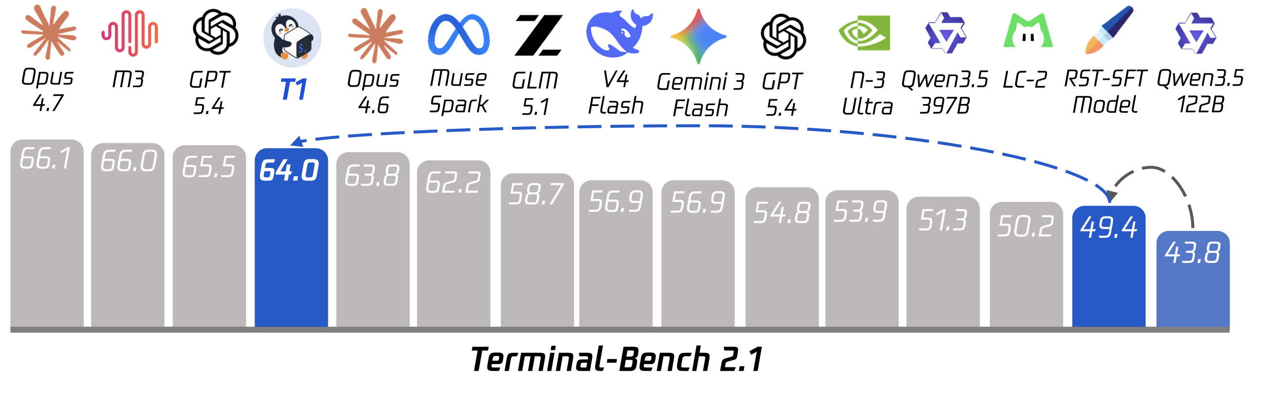
图 9|T1 在 Terminal-Bench 2.1 上的站位。蓝色柱是我们自己的流水线: base 模型(43.8)、我们初始化所用的 SFT checkpoint(49.4)、RL 之后的 T1(64.0); 虚线箭头标出两个阶段——SFT 贡献 +5.6 pp,RL 再贡献 +14.6 pp。灰色柱是对比模型。 步长对比才是实质性的论点:从 base 到最终大约四分之三的距离是靠终端任务上的强化学习赚来的, 而不是靠对示范的模仿。只做 SFT 会让它在图里倒数第二,低于每一个对比项; 同一份权重经过 RL 后总体排到第四,并超过 Claude Opus 4.6——而它只有 10B 激活参数。
Figure 9 | Terminal-Bench 2.1 standing of T1. Blue bars trace our own pipeline: the base model (43.8), the SFT checkpoint we initialize from (49.4), and T1 after RL (64.0); the dashed arrows mark the two stages — +5.6 pp from SFT and a further +14.6 pp from RL. Grey bars are the comparison models. The contrast in step sizes is the substantive claim: roughly three-quarters of the total distance from base to final is earned by reinforcement learning on terminal tasks rather than by imitation of demonstrations. Supervised fine-tuning alone leaves it second from last, below every comparison entry, while the same weights after RL land fourth overall and above Claude Opus 4.6 — with 10B active parameters.
Held-out benchmark over training steps
图 10|留出 Terminal-Bench 2.1 解决率随训练步的变化。 实心标记是被评测的 checkpoint(每 10 个 rollout 步一次),星标是峰值;两条虚线是固定锚点 ——base(43.8%)和初始化所用的 SFT(49.4%)。三个特征值得点名: 增益是立刻发生的(第 9 步已达 56.2%,到前沿带的大部分距离在前十分之一的训练里就走完了); 中段是平台而非下滑(第 19–59 步落在 55.1–57.3% 的带内,跨度约相当于 89 个任务中的 3 个, 在评测噪声之内,而这个带的下沿仍高出 SFT 5.7 pp); 两次阶跃出现得很晚,在第 69 步(61.8%)和第 109 步(64.0%) ——而这也正是解释方差最高的时候:只有当 critic 成为一个校准良好的基线,actor 才能做出它最大的可用跳跃
Figure 10 | Held-out Terminal-Bench 2.1 resolved rate over the production run. Filled markers are the evaluated checkpoints (every 10 rollout steps), the starred point is the peak; the dashed rules are the two fixed anchors, the base model (43.8%) and the SFT checkpoint the run is initialized from (49.4%). Three features are worth naming. The gain is immediate: step 9 is already at 56.2%, so most of the distance to the frontier band is covered in the first tenth of the run. The middle is a plateau, not a decline: steps 19–59 sit in a 55.1–57.3% band whose spread is about three tasks out of 89 — within evaluation noise — and the floor of that band still stands 5.7 pp above SFT. The two step-changes arrive late, at step 69 (61.8%) and step 109 (64.0%), which is also where explained variance is highest: the actor makes its largest usable jumps only once the critic has become a well-calibrated baseline.
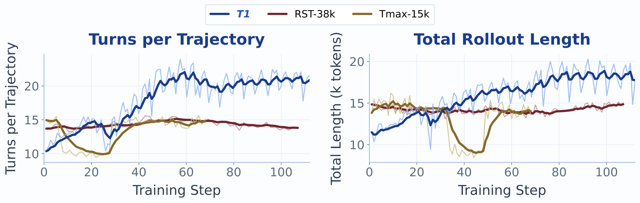
Behavioral dynamics: turns and sequence length
图 11|行为动态。:每条轨迹的平均工具调用轮数。:每条轨迹的总序列长度。 两者在训练中大致翻倍(轮数 10.4 → 20.9,长度 11.5k → 17.8k token),随后趋平而非无界增长。 我们把它读作测试计数奖励的预期效果而非长度作弊,理由有三:增长是有界的 (两条曲线在约第 60 步后走平,最后三分之一训练几乎没有增加), 而那个失败的加性长度惩罚产生的是完全相反的特征——从 22 无界涨到 50+; 平台落在约 21 轮,仍远在 60 轮的 harness 预算之内; 并且增长与奖励、基准增益是同时发生而非与之脱钩的 ——在验证器含有许多可独立检查断言的任务上,多几轮换来的确实是多几个通过的测试。
Figure 11 | Behavioral dynamics. Left: average tool-call turns per trajectory. Right: total sequence length per trajectory. Both roughly double over training (turns 10.4 → 20.9, length 11.5k → 17.8k tokens) and then flatten rather than growing without bound. We read this as the intended effect of the test-count reward rather than length hacking, for three reasons: the growth is bounded (both curves flatten after roughly step 60 and the last third of training adds essentially nothing), whereas the failed additive length penalty produced exactly the opposite signature — unbounded growth from 22 to 50+ turns; the plateau lands at ~21 turns, still well inside the 60-turn harness budget; and the growth is concurrent with the reward and benchmark gains rather than decoupled from them — on tasks whose verifiers contain many independently checkable assertions, more turns here buy more passing tests.

残余失败长什么样How the remaining failures look

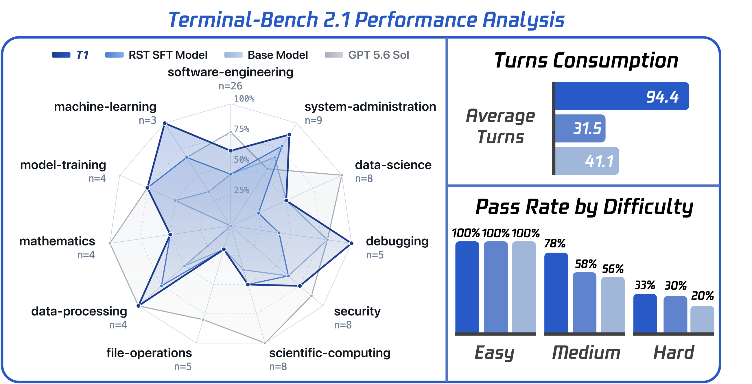
针对 GPT-5.6 的失败分析被难任务上的 Agent 超时所主导: 在六个代表性的未解决任务上,我们的 Agent 花了 164–473 轮,而 GPT-5.6 只花 6–40 轮; 另有三个因沙箱错误失败。评测约束本身也是不对称的 ——我们最大输入 56k 而对方 120k、最大输出 8,192 而对方 32,768、thinking 关闭而对方中等推理强度 ——所以差距的一部分是预算而非能力。所有失败中只有 4 个撞到 500 轮的评测天花板,11 个有部分子测试通过; 分析表的结论是:大多数失败是「方向错了」,而不是「差一点就成」。

The failure analysis against GPT-5.6 is dominated by agent timeouts on hard tasks: on six representative unsolved tasks our agent spent 164–473 turns where GPT-5.6 spent 6–40, and three more failed on sandbox errors. The evaluation constraints were also asymmetric — ours ran with max input 56k vs their 120k tokens, max output 8,192 vs 32,768, thinking off vs medium reasoning effort — so part of the gap is budget, not capability. Of all failures, only 4 hit the 500-turn evaluation ceiling and 11 had partial sub-test passes; the analysis' own conclusion is that most failures are "wrong direction", not "almost done".

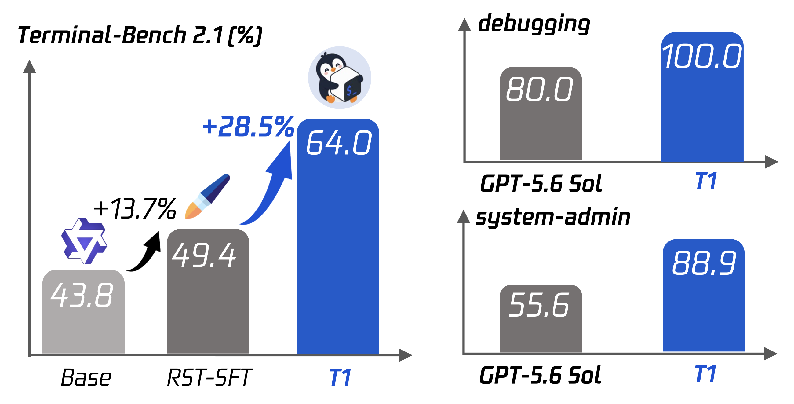
Stage-wise gains and per-domain comparison
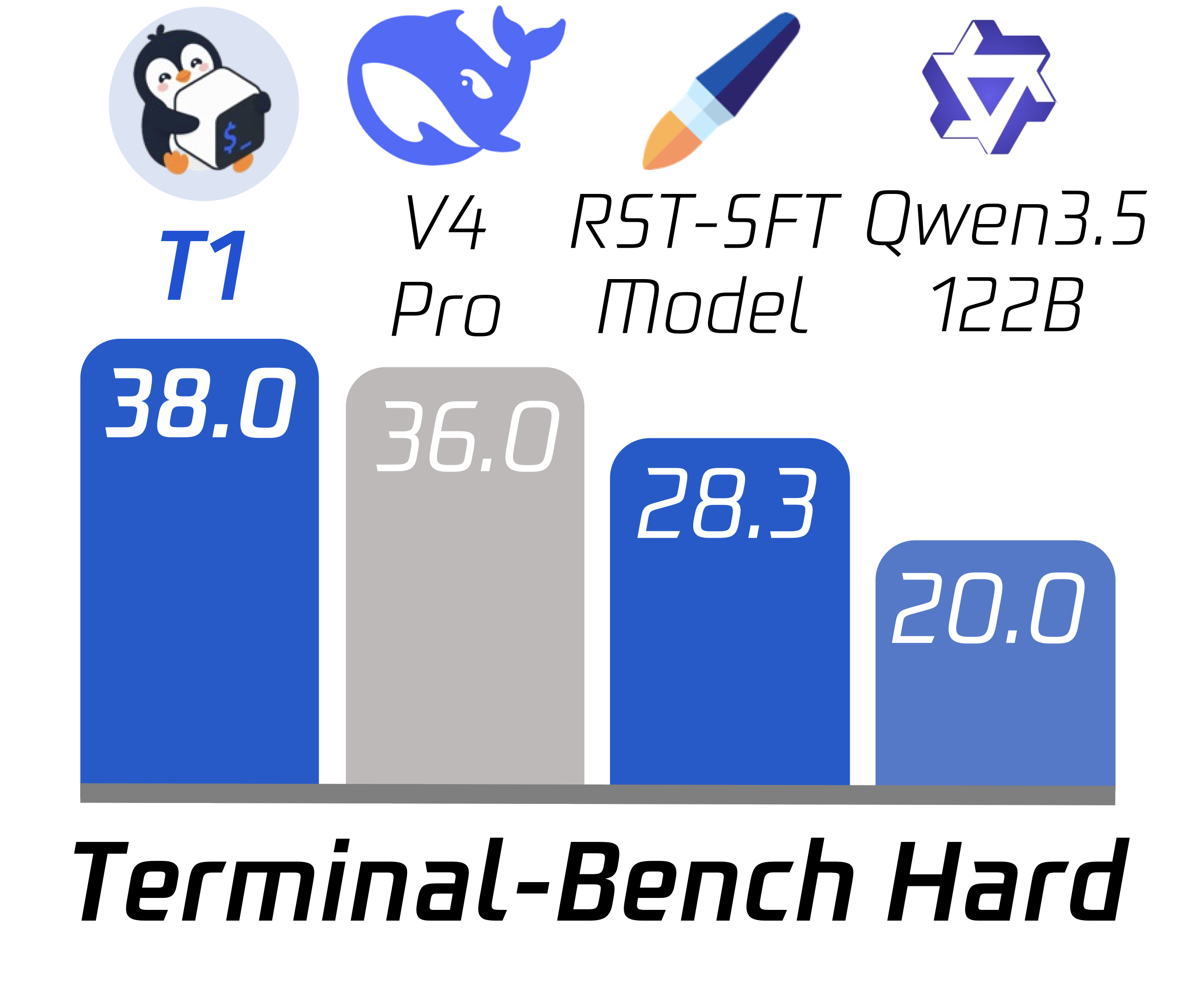
图 12|:总增益按阶段分解。SFT 把 base 从 43.8% 抬到 49.8%(相对提升 13.7%), RL 再把 SFT 抬到 64.0%(相对提升 28.5%)——即强化学习阶段贡献了约两倍于监督阶段的相对增益。 :分领域对比。对 GPT-5.6 Sol,我们在调试子集上是 100.0 对 80.0, 在系统管理上是 88.9 对 55.6,在这两个领域上直接超过一个更强的通用专家模型。 而这两类恰好是最依赖「读失败的测试 → 形成假设 → 跑命令 → 修正」这种长链多步推理与工具使用交错的任务族, 也正是终端 Agent RL 循环所优化的能力。补集同样有信息量: 失败集中在 Strategy-15k 覆盖很薄的 ML / 数据科学 / 科学计算任务上, 说明剩余头部空间很大程度上是训练池覆盖度问题,而不是 Agent 推理循环的问题。
Figure 12 | Left: the total gain decomposed by stage. SFT lifts the base model from 43.8% to 49.8%, a 13.7% relative improvement, and RL then lifts SFT to 64.0%, a further 28.5% relative improvement — the reinforcement-learning stage contributes roughly twice the relative gain of the supervised stage. Right: per-domain comparison. Against GPT-5.6 Sol we reach 100.0 versus 80.0 on the debugging subset and 88.9 versus 55.6 on system administration, surpassing a stronger general-purpose expert model outright on these two domains. Both are precisely the task families that depend on long chains of multi-step reasoning interleaved with tool use — read a failing test, form a hypothesis, run a command, revise — which is exactly the competence the terminal-agent RL loop optimizes. The complement is equally informative: failures concentrate in ML / data-science / scientific-computing tasks that Strategy-15k covers only thinly, indicating that the remaining headroom is largely a matter of training-pool coverage rather than of the agent's reasoning loop.
对有效性的威胁(我们自己先说)Threats to validity (stated up front)

表 1 里「二值 vs 稠密」的对比是实验级对比,不是单轴消融:在 TMax 与 Strategy-15k 两次实验之间,奖励、数据池、初始化(base vs RST)、critic 温度(冷 vs 热)、 上下文墙(64k vs 84k)和 R³(关 vs 开)这五六个轴是同时变化的。 稠密奖励的读解是被支持的——同一份稠密配方在两个不同数据池上从 RST 出发都有效, 而二值配方在 SFT 之下就平台了——但一次同池、同初始化、R³ 对齐的受控消融尚未做过。 评测方差在第 109 步的重复中可见(0.596–0.635):单次评测中小于约 3 个点(约 3 个任务)的差异不应被过度解读。

The binary-versus-dense comparison in Table 1 is a campaign comparison, not a single-axis ablation: between the TMax and Strategy-15k runs the reward, the data pool, the initialization (base vs RST), the critic temperature (cold vs warm), the context walls (64k vs 84k) and R³ (off vs on) all change together. The dense-reward reading is supported — the same dense recipe works from RST on two different pools while the binary recipe plateaued below SFT — but a controlled, same-pool, same-init, R³-matched ablation has not been run. Evaluation variance is visible in the iteration-109 repeats (0.596–0.635): single-eval differences under ~3 points (about 3 tasks) should not be over-interpreted.

08基础设施:把两个 122B 塞进同一批卡Infrastructure: two 122B models per GPU set

带独立 critic 的 PPO 意味着每一张「actor 卡」实际上要托管两个 122B 模型 (靠强制 offload 分时复用),每一个单独都必须装进 95 GiB。最初的 56 卡拓扑活过了 critic-only 阶段, 却在第一个 actor + critic 联合步上崩了:在 critic 的 GatedDeltaNet 前向里, 已用 90.56 GiB 的情况下再申请 632 MiB。

PPO with a separate critic means every "actor GPU" hosts two 122B models (time-multiplexed by forced offload); each alone must fit in 95 GiB. The initial 56-GPU topology survived critic-only steps and crashed at the first joint actor+critic step, in the critic's GatedDeltaNet forward: a 632 MiB allocation with 90.56 GiB already in use.

我们的做法是建立一个按显存标定的模型,直接对着真实崩溃点校准,并和拓扑预设一起放在启动脚本里。 它预测的崩溃点与实测相差 0.1 GB 以内。三个结构性事实从中掉出来,并且每一个都被验证过:

We built a per-GPU memory model, calibrated against the real crash and kept in the launch script alongside the topology presets. It predicted the observed crash to within 0.1 GB. Three structural facts fall out, each of which was verified:

为此我们给 GatedDeltaNet 补上了原生上下文并行:它的递归扫描在通用路径里不是 CP-safe 的, 历史上因此被钉在 1,让最差单条轨迹的激活成了 OOM 的墙(实测约 330 KiB/token,是最初估计的 4 倍 ——这也是早期显存预测系统性偏低的原因)。改造后每个 rank 只算一部分 token 并传递递归状态, 并显式处理了「slime 按 zig-zag 排布分片、而底层算子期望连续分片」这个错位。 GPU 测试验证了前向逐位一致、梯度最大差 1.2 × 10⁻⁷,激活峰值从 10.57 GB 降到 CP4 下的 2.70 GB(3.92 倍)。这正是 84k 训练墙可行的前提。

We therefore added native context parallelism for GatedDeltaNet: its recurrent scan is not CP-safe in the generic path, so CP was historically pinned to 1, making the worst single trajectory's activation the OOM wall (measured at ~330 KiB/token, 4× the original estimate — the reason early memory projections were systematically low). After the change each rank computes a slice of tokens and passes recurrent state, with an explicit relayout for the mismatch between slime's zig-zag shard layout and the contiguous shards the underlying kernels expect. GPU tests verify forward bit-exactness against the single-rank reference and gradient max-diff 1.2 × 10⁻⁷; activation peaks drop from 10.57 GB to 2.70 GB at CP4 (3.92×). This is what makes the 84k training wall feasible.

在 128 卡、每步约一小时的规模上,「罕见」故障是每次实验的必然事件。我们针对四类故障做了加固: 死掉的推理引擎(健康探针 + 在下次权重同步时重建)、无界的控制面 HTTP(有界超时,但批量权重传输故意保持无界)、 watchdog 把慢 rank 误判成死锁(重建的 NCCL 组默认 30 分钟、CP > 1 的配方 120 分钟, Gloo 控制组 60 分钟)、以及文件描述符耗尽(320 个并发沙箱试验把协调进程顶过 1024 的软限制, rollout 于是永远停在「收集到 0 个」而没有任何报错)。 检查点是有意不对称的:只存权重、每 10 步一次——更小更快, 代价是崩溃意味着重启而不是续跑,这个代价被明确记录并接受。

At 128 GPUs and ~1 hour per step, "rare" failures are per-run certainties. We hardened four classes: dead inference engines (health pings + recreation at the next weight sync), unbounded control-plane HTTP (bounded timeouts, while bulk weight transfers deliberately stay unbounded), watchdog-versus-straggler misclassification (recreated NCCL groups default to 30 min, 120 min in CP > 1 recipes, and the Gloo control group to 60 min), and file-descriptor exhaustion (320 concurrent sandbox trials pushed the coordinator past the 1024 soft limit, after which rollout collection sat forever at "collected 0" with no error). Checkpointing is asymmetric by choice: weights-only, every 10 steps — smaller and faster, at the documented cost that a crash means restart rather than resume.

沙箱层在 512 路并发下也有自己的工程:试验由绑定在 rollout 节点上的 Ray 辅助 worker 托管, 让试验流量不经过协调进程;沙箱创建被一个异步令牌桶限速到 6/s 以匹配云厂商的配额; skim 过采样每步启动 560 个试验、接受最先完成的 512 组、取消尾部—— 这既是吞吐的来源,也是我们认为最重要的待解权衡: 被取消的尾部恰好集中了最难的任务族,这是一个公开承认的选择偏差风险。

The sandbox layer at 512-way concurrency has its own engineering: trials are hosted by per-node Ray auxiliary workers pinned to rollout nodes, keeping trial traffic off the coordinator; sandbox creation is paced by an async token bucket at 6/s against the provider's quota; and skim-oversampling launches 560 trials per step, accepts the first 512 completed groups and cancels the tail. This is both the source of throughput and what we consider the most important open trade-off: the cancelled tail concentrates precisely the hardest task families, an openly acknowledged selection-bias risk.

09踩过的坑Lessons learned

我们把失败记录得足够细,以便复用。每一条都给出症状、当初错误的第一假设,以及真正的机制。

We record the failures in enough detail to be reusable. Each item names the symptom, the wrong first hypothesis where we had one, and the actual mechanism.

伪装成别的故障的故障Failures that impersonated other failures

静默损坏陷阱Silent-corruption traps

我们刻意做的事Things we chose not to do

KL 正则和熵奖励关闭(裁剪本身已足够约束更新;而在 R³ 下 actor 与 reference 的 KL 按设计非零,用它会正则错方向); TIS 修正只测量不施加到损失;RL 期间关闭 MoE 辅助负载均衡损失; expandable_segments 保持关闭(与 PPO 所需的 offload 内存节省器不兼容); 稠密奖励实验的 checkpoint 只存权重——崩溃意味着重启,这是为了在 122B 规模上换取保存速度而接受的代价。

KL regularization and entropy bonuses are off (the clip alone constrains updates; and under R³ the actor/reference KL is nonzero by design and would mis-regularize); TIS correction is measured but not applied to the loss; the MoE auxiliary load-balancing loss is off during RL; expandable_segments stays off because it is incompatible with the memory-saver offload PPO requires; and the dense-reward run's checkpoints are weights-only — a crash means restart, an accepted trade for save speed at 122B scale.

10局限与后续Limitations and future work